Abaqus tutorial: Learn FEM, Applications, Advantages, and Solvers

What is Finite Element Method (FEM)?

FEM engineering is an numerical methodology employed to address a wide range of physics and engineering problems. The finite element approach is applied to solve problems in various fields of engineering and mathematical physics, including structural analysis, heat transfer, fluid flow, mass transport, and electromagnetic potential. Analytical mathematical solutions are often unattainable for modeling the behavior of physical systems with complex geometries, loadings, and material properties. The complexity introduced by these factors renders the solution of the corresponding differential equations impractical.

To overcome this challenge, numerical techniques such as the finite element approach are utilized to approximate the solutions of these equations. Instead of directly solving the differential equations, the problem is formulated in the finite element method as a system of simultaneous algebraic equations. These numerical techniques estimate the unknown values at discrete locations along the continuum, allowing for the representation of the system’s behavior.

Abaqus is one of the software that uses the FEM.

FEM applications

Both structural and nonstructural issues can be examined using the finite element method.

The most typical structural areas are:

Stress analysis, including truss and frame analysis
Buckling, such as in columns, frames, and vessels
Vibration analysis, such as in vibratory equipment
Impact problems, including crash analysis of vehicles

And nonstructural problems include:

Heat transfer, such as in electronic devices emitting heat as in a personal computer microprocessor chip
Fluid flow, including seepage through porous media
Distribution of electric or magnetic potential

FEM advantages

As mentioned earlier, the finite element method, also known as finite element analysis, has been widely employed to address various structural and nonstructural problems. This method offers several advantages over traditional approximate methods used for modeling and determining physical quantities such as displacements, stresses, temperatures, pressures, and electric currents. These advantages stand in contrast to conventional methods taught in traditional material mechanics and heat transfer courses. The key advantages include:

Easy handling of bodies with irregular shapes in the design process.
Ability to handle stress and strain cases without difficulty.
Capability to model bodies consisting of different materials by evaluating each element equation separately.
Flexibility in managing a wide range of boundary conditions.
Ability to resize components as needed and incorporate higher-order elements in the finite element model.
Simplicity in simulating various material qualities from element to element or even within a single element.
Accessibility and popularity within the engineering community due to its user-friendly nature, compactness, and emphasis on results.
Capability to handle nonlinear behavior arising from significant deformations and material properties by incorporating a finite element model.
Availability of a variety of computer software programs and books, making the finite element method a flexible and effective numerical approach.

These advantages contribute to the widespread use and acceptance of the finite element method in engineering, as it offers a practical and versatile solution to a broad range of problems.

FEM disadvantages

There are several limitations associated with the finite element method (FEM):

The mesh used for nodal analysis requires a substantial amount of input data.
Achieving an exact idealization of complex shapes for real-life objects is challenging.
The implementation of FEM is intricate and primarily relies on computer-based computations.
The time required for solving problems increases as the mesh becomes finer, resulting in longer computation times.
The output results obtained from FEM can vary significantly. While FEM provides an approximate solution, efforts are made to minimize errors across the entire domain. However, the exact solution is only achieved at the nodes.

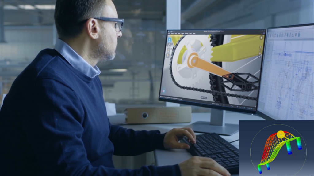
What is Abaqus CAE?

Abaqus CAE is a comprehensive suite of advanced engineering simulation programs that utilize the finite element method to address a wide range of problems, ranging from simple linear analyses to intricate nonlinear simulations. With Abaqus software, users gain access to an extensive library of elements for modeling diverse geometries, as well as a broad selection of material models capable of simulating the behavior of various common engineering materials. These materials include metals, rubber, polymers, composites, reinforced concrete, crushable and resilient foams, as well as geotechnical materials like soils and rock.

While originally designed as a versatile simulation tool primarily focused on structural problems involving stress and displacement, Abaqus software can also be utilized for investigating other areas of interest. These include heat transfer, mass diffusion, thermal management of electrical components through coupled thermal-electrical analyses, acoustics, soil mechanics through coupled pore fluid-stress analyses, and piezoelectric analysis.

Abaqus/CAE is a software utilized for both pre-processing, involving the modeling and analysis of mechanical parts and assemblies, and post-processing, which involves examining the results of finite element analysis. This software is widely employed in industries such as automotive, aerospace, and industrial products due to its extensive material modeling capabilities and flexibility. Users can even create their own material models, enabling simulation of novel materials within Abaqus software. Beyond academic and research institutions, Abaqus software is also favored by non-academic engineering institutes.

Abaqus software is particularly well-suited for production-level simulations that require coupling across multiple fields. It offers a broad array of multi-physics capabilities, including the coupling of acoustic-structural interactions, piezoelectric effects, and structural-pore interactions. This versatility makes it an ideal solution for complex simulations that involve diverse physical phenomena.

System of units in Abaqus

Beginner users often find it perplexing that quantities in Abaqus, and similar finite element programs like Ansys and LS-Dyna, do not have explicit units. This discrepancy can lead to confusion when dealing with measurements such as stress or when specifying parameters like Young’s modulus or density. To gain clarity on how units are handled in Abaqus, it is recommended to read a post that explains Abaqus units and refer to the Abaqus units table provided at the end.

It’s important to note that the absence of explicit units in these programs is not unique to Abaqus but is a standard practice across many finite element software. Consequently, it becomes the user’s responsibility to ensure the consistent use of units for the provided numbers to maintain accuracy and avoid errors.

In Abaqus, except for rotation and angle measures, there are no predefined units. Consequently, it is crucial to select units that are internally consistent. This implies that derived units within the chosen system should be expressed in terms of fundamental units without the need for conversion factors. To gain a comprehensive understanding of Abaqus units or the concept of units in Abaqus, it is recommended to read a helpful article that provides sufficient information within a four-minute read.

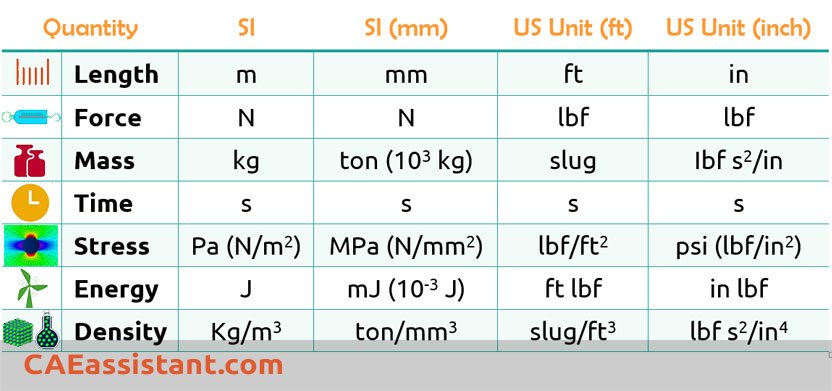
In a general sense, a consistent system of units comprises fundamental units, including Length (L), Mass (M) or Force (F), and Time (T), which serve as the base units. Additionally, there are derived units, which are formed by manipulating the base units through powers, products, or quotients. These derived units can be numerous and have the potential for unlimited variability.

Below is a table showcasing various examples of consistent systems of units. Each system includes the mass density and Young’s modulus of steel as reference values. The term “GRAVITY” represents the gravitational acceleration. This table is referred to as the Abaqus units table.

Before we continue, if you are interested to learn Abaqus software from the beginning to advanced level, you can visit this Abaqus tutorial page.

What are Abaqus Explicit and Implicit solvers?

These solvers in FEM analysis are based on two different approaches: implicit (used in Abaqus/Standard) and explicit. Understanding the distinction between these two numerical approaches helps in determining which solver to utilize.

In the implicit method, equilibrium is maintained between externally applied loads and internally generated reaction forces at each solution step using the Newton-Raphson method. On the other hand, the explicit method does not enforce equilibrium. However, this doesn’t imply that the explicit method lacks accuracy. By increasing the number of solution steps, i.e., reducing the time step size, the deviation from equilibrium can be minimized to nearly zero.

Here are the key differences:

Implicit method is unconditionally stable.

Implicit approach is both incremental and iterative, while the explicit approach is only incremental.

Implicit method is more computationally expensive per increment, whereas explicit method is relatively cheaper. Additionally, the disk space and memory usage required for explicit method are typically smaller compared to implicit method.

As the size of the model increases, the explicit method exhibits significant cost savings over the implicit method.

These differences highlight the contrasting characteristics of the implicit and explicit approaches, including stability, computational requirements, and cost considerations, which are important factors to consider when selecting the appropriate solver for a given analysis.